Microsoft Excel is a powerful tool for data processing with tables and charts. One of its most valuable features is the wide variety of functions available, allowing users to automate calculations, analyze data, and simplify tasks. In this article, we will explore 25 essential Excel functions that can significantly improve your proficiency in Excel.
Using Functions in Excel
Before proceeding, there are three easy ways to use functions in Excel.
- Type = in any cell and start typing your function. Excel will show the list of available functions and the syntax for the selected item.
- Click the “Insert function” (fx) icon showing left side of the formula bar. This will open a pop-up with a list of all Excel functions using which you can create complex formulae. You can also search or filter the functions based on category.
- Select a cell containing a function and click on the fx icon to see all the arguments and acceptable values you can use in the syntax of that function.

25 Most Useful Excel Functions with Syntax
Below is the summary of top 25 Excel functions with their syntax. The arguments within [ ] are optional to use in the function.
| Function | Syntax | Description |
|---|---|---|
| SUM | =SUM(number1, [number2], …) | Adds up values within a specified range. |
| TODAY | =TODAY() | Returns the current date, updating automatically. |
| NOW | =NOW() | Returns the current date and time, updating automatically. |
| AVERAGE | =AVERAGE(number1, [number2], …) | Calculates the mean (average) of a set of numbers. |
| SORT | =SORT(array, [sort_index], [sort_order], [by_col]) | Sorts a range or array in ascending or descending order. |
| TRANSPOSE | =TRANSPOSE(array) | Converts rows to columns (or vice versa). |
| UNIQUE | =UNIQUE(array, [by_col], [exactly_once]) | Returns unique values from a range or array, filtering out duplicates. |
| XLOOKUP | =XLOOKUP(lookup_value, lookup_array, return_array, [if_not_found], [match_mode], [search_mode]) | Searches for a value and returns a corresponding value from another column. |
| XMATCH | =XMATCH(lookup_value, lookup_array, [match_mode], [search_mode]) | Returns the position of a specified value in a range or array. |
| CONCAT | =CONCAT(text1, [text2], …) | Joins multiple strings or text values into one. |
| EXACT | =EXACT(text1, text2) | Checks if two text strings are exactly the same, case-sensitive. |
| LEFT | =LEFT(text, [num_chars]) | Extracts a specified number of characters from the beginning of a text string. |
| PROPER | =PROPER(text) | Converts text to proper case, capitalizing the first letter of each word. |
| REPLACE | =REPLACE(old_text, start_num, num_chars, new_text) | Replaces part of a text string with another string. |
| RIGHT | =RIGHT(text, [num_chars]) | Extracts a specified number of characters from the end of a text string. |
| TRIM | =TRIM(text) | Removes extra spaces from text, except for single spaces between words. |
| ENCODEURL | =ENCODEURL(text) | Encodes text for safe use in web addresses (URL encoding). |
| CONVERT | =CONVERT(number, from_unit, to_unit) | Converts a number from one measurement unit to another. |
| NOT | =NOT(logical) | Reverses a logical value; returns TRUE for FALSE and vice versa. |
| OR | =OR(logical1, [logical2], …) | Returns TRUE if any of the provided conditions are TRUE. |
| DELTA | =DELTA(number1, [number2]) | Compares two numbers and returns 1 if they’re equal, otherwise 0. |
| AND | =AND(logical1, [logical2], …) | Returns TRUE if all provided conditions are TRUE. |
| CELL | =CELL(info_type, [reference]) | Provides information about a cell, such as its address, contents, or format. |
| TYPE | =TYPE(value) | Returns the data type of a value: 1 for numbers, 2 for text, 4 for logical values, etc. |
| IF | =IF(condition, value_if_true, value_if_false) | Checks a condition and returns one value if TRUE and another if FALSE. |
Explanation with Examples
Here’s a detailed guide on using 25 of Excel’s most practical functions, complete with examples and explanations.
1. SUM
Syntax:
=SUM(number1, [number2], …)Example:
=SUM(D1:D10)Explanation:
Sum function adds up values within a specified range. For instance, using =SUM(D1:D10) will calculate the total of cells D1 through D10.

2. TODAY
Syntax:
=TODAY()Example:
=TODAY()Explanation:
Returns the current date. Useful for tracking timelines without manually updating the date each day. For instance, =TODAY() might show “2025-11-09” if today’s date is November 9, 2025. The date format will be used as per your system’s setup.

3. NOW
Syntax:
=NOW()Example:
=NOW()Explanation:
Returns the current date and time, updating automatically. Use =NOW() for current timestamp that updates on every calculation.

4. AVERAGE
Syntax:
=AVERAGE(number1, [number2], …)Example:
=AVERAGE(D1:D3)Explanation:
Calculates the mean of a set of numbers. If cells D1 through D3 contain test scores, =AVERAGE(D1:D3) will return their average.

5. SORT
Syntax:
=SORT(array, [sort_index], [sort_order], [by_col])Example:
=SORT(D1:D5, 1, 1)
=SORT(D1:D5, 1, -1)Explanation:
Sorts a range of data in ascending or descending order. These examples will sort values in cells D1 through D5 in ascending and descending orders.


6. TRANSPOSE
Syntax:
=TRANSPOSE(array)Example:
=TRANSPOSE(D1:E5)Explanation:
Converts rows to columns and vice versa. For example, =TRANSPOSE(D1:E5) will make the data to H1:L2 as shown below.

7. UNIQUE
Syntax:
=UNIQUE(array, [by_col], [exactly_once])Example:
=UNIQUE(D1:D10)Explanation:
Filters a list to show only unique values. Using =UNIQUE(D1:D10) in the below example will make a list only with unique values.

8. XLOOKUP
Syntax:
=XLOOKUP(lookup_value, lookup_array, return_array, [if_not_found], [match_mode], [search_mode])Example:
=XLOOKUP("Apple",D1:D7,E1:E7)
=XLOOKUP("Grapes",D1:D7,E1:E7,"Not Found")Explanation:
This is a combination HLOOKUP and VLOOKUP functions searches for a value in one column and returns a corresponding value from another column. With the first example, it will return 10 corresponding to the looked-up value “Apple” and with the second example, it will return “Not Found”.

9. XMATCH
Syntax:
=XMATCH(lookup_value, lookup_array, [match_mode], [search_mode])Example:
=XMATCH("Banana",D1:D7,2,1)Explanation:
Returns the position of a specified value. Find the position of “Banana” in the array D1:D7 and returns its position as 6. In the example, match mode 2 indicates wildcard search character match and search mode 1 indicates searching first-to-last.

10. CONCAT
Syntax:
=CONCAT(text1, [text2], …)Example:
=CONCAT(C1," ",D1," ",E1)Explanation:
Joins multiple strings into one. If C1 is “Apple”, D1 is “is” and E1 is “good”, then =CONCAT(C1,” “,D1,” “,E1) returns “Apple is good.”

11. EXACT
Syntax:
=EXACT(text1, text2)Example:
=EXACT(C1, D1)Explanation:
Checks if two text strings are identical. If C1 has “Apple” and D1 has “Orange,” it will return FALSE. Note that this function is case-sensitive.

12. LEFT
Syntax:
=LEFT(text, [num_chars])Example:
=LEFT(C1, 4)Explanation:
Extracts characters from the beginning of a string. If cell C1 contains “Pineapple”, =LEFT(C1, 4) returns “Pine”.

13. PROPER
Syntax:
=PROPER(text)Example:
=PROPER(C1)Explanation:
Converts text to proper case by capitalizing the first letter of each word. For “hello world,” it returns “Hello World”.

14. REPLACE
Syntax:
=REPLACE(old_text, start_num, num_chars, new_text)Example:
=REPLACE(A1, 1, 3, "New")Explanation:
Replaces part of a text string. If A1 is “Old Text,” =REPLACE(A1, 1, 3, “New”) changes it to “New Text.”

15. RIGHT
Syntax:
=RIGHT(text, [num_chars])Example:
=RIGHT(C1, 5)Explanation:
Extracts characters from the end of a string. If C1 is “Pineapple”, =RIGHT(C1, 5) returns “apple”.

16. TRIM
Syntax:
=TRIM(text)Example:
=TRIM(C1)Explanation:
Removes extra spaces from text, keeping only single spaces between words. Helpful when cleaning data from inconsistent sources.

17. ENCODEURL
Syntax:
=ENCODEURL(text)Example:
=ENCODEURL(C1)Explanation:
Encodes a URL to be safely used in web addresses. Useful when you need to send URLs through external programs or APIs.

18. CONVERT
Syntax:
=CONVERT(number, from_unit, to_unit)Example:
=CONVERT(30, "cm", "in")Explanation:
Converts a number from one measurement unit to another. =CONVERT(30, “cm”, “in”) changes 30 centimeters to inches which is 11.81102362.

19. NOT
Syntax:
=NOT(logical)Example:
=NOT(C1=10)Explanation:
Reverses a logical value. If C1 equals 10, =NOT(C1=10) will return FALSE and =NOT(C1=9) will return TRUE.

20. OR
Syntax:
=OR(logical1, [logical2], …)Example:
=OR(C1=20,D1<30)Explanation:
Checks if any of the conditions are true. If C1 is 20 or D1 is less than 30, it returns TRUE.

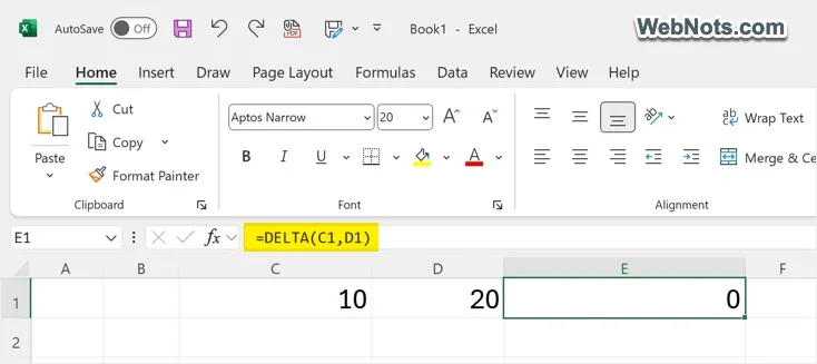
21. DELTA
Syntax:
=DELTA(number1, [number2])Example:
=DELTA(C1, D1)Explanation:
Compares two numbers and returns 1 if they are equal, otherwise 0. Useful for condition-based checks.
22. AND
Syntax:
=AND(logical1, [logical2], …)Example:
=AND(C1>19,D1<16)Explanation:
Checks if all conditions are true. Returns TRUE only if both C1 is greater than 19 and D1 is less than 16.

23. CELL
Syntax:
=CELL(info_type, [reference])Example:
=CELL("address", C1)Explanation:
Returns information about a cell, like its address, content, or format. =CELL(“address”, C1) shows the cell’s address like $C$1.

24. TYPE
Syntax:
=TYPE(value)Example:
=TYPE(C1)Explanation:
Identifies the data type in a cell: 1 for numbers, 2 for text, 4 for logical values, etc. Useful in complex data analysis.

25. IF
Syntax:
=IF(condition, value_if_true, value_if_false)Example:
=IF(C1>10, "YES", "NO")Explanation:
Checks a condition and returns one value if true and another if false.

Conclusion
These 25 essential Excel formulas are the foundation of mastering Excel. Whether you are analyzing data, preparing reports, or automating repetitive tasks, these formulas will save time and boost your productivity.